Note
Go to the end to download the full example code.
New grid systems: Plus codes, Maidenhead, and GARS.#
This example demonstrates the new grid systems added to M3S: Plus codes (Open Location Code), Maidenhead locator system, and GARS (Global Area Reference System).
Testing coordinates: 37.7749, -122.4194 (San Francisco)
============================================================
1. Plus codes (Open Location Code)
----------------------------------------
Plus code: 48V9+HQJF
Cell area: 0.0611 km²
Precision: 4
Number of neighbors: 8
2. Maidenhead Locator System
----------------------------------------
Maidenhead locator: CM87SS
Cell area: 33.9295 km²
Precision: 3
Number of neighbors: 8
3. GARS (Global Area Reference System)
----------------------------------------
GARS identifier: 116JV3
Cell area: 609.8944 km²
Precision: 2
Number of neighbors: 8
4. Bounding Box Queries
----------------------------------------
Bounding box: (37.67, -122.52) to (37.87, -122.32)
Plus codes cells in bbox: 6561
Maidenhead cells in bbox: 20
GARS cells in bbox: 4
5. Precision Comparison
----------------------------------------
Plus codes:
Precision 1: 48 (area: 3746070.4678 km²)
Precision 2: 48V9+ (area: 9806.4958 km²)
Precision 3: 48V9+HQ (area: 24.4282 km²)
Precision 4: 48V9+HQJF (area: 0.0611 km²)
Maidenhead:
Precision 1: CM (area: 2030598.6063 km²)
Precision 2: CM87 (area: 19612.7501 km²)
Precision 3: CM87SS (area: 33.9295 km²)
Precision 4: CM87SS95 (area: 0.3393 km²)
GARS:
Precision 1: 116JV (area: 2443.7115 km²)
Precision 2: 116JV3 (area: 609.8944 km²)
Precision 3: 116JV37 (area: 67.8402 km²)
6. GeoDataFrame Integration
----------------------------------------
Plus codes intersect result: 1 cells
Cell ID: 48V9+HQJF
Maidenhead intersect result: 1 cells
Cell ID: CM87SS
GARS intersect result: 1 cells
Cell ID: 116JV3
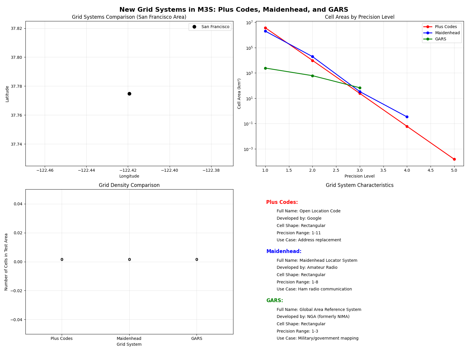
=== Creating Grid Systems Visualization ===
/home/runner/work/m3s/m3s/examples/new_grids_example.py:286: UserWarning: Attempting to set identical low and high ylims makes transformation singular; automatically expanding.
ax3.set_ylim(0, max(cell_counts) * 1.1)
Grid comparison plots saved as 'new_grids_comparison.png'
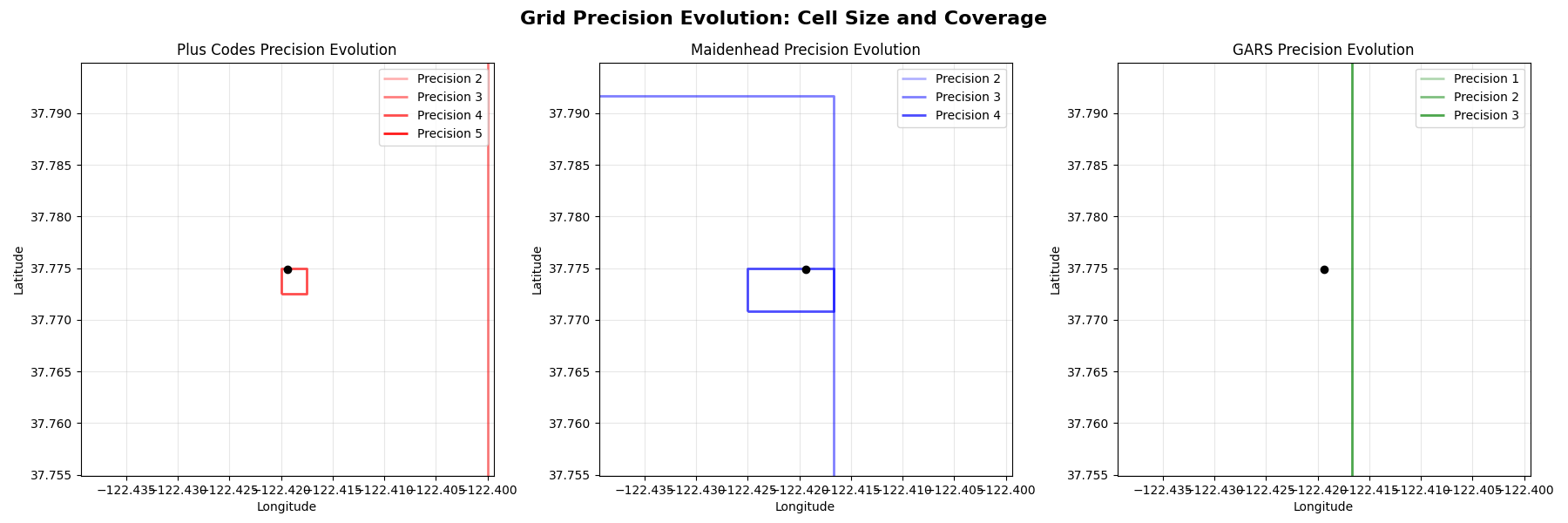
=== Creating Precision Evolution Plots ===
Precision evolution plots saved as 'precision_evolution.png'
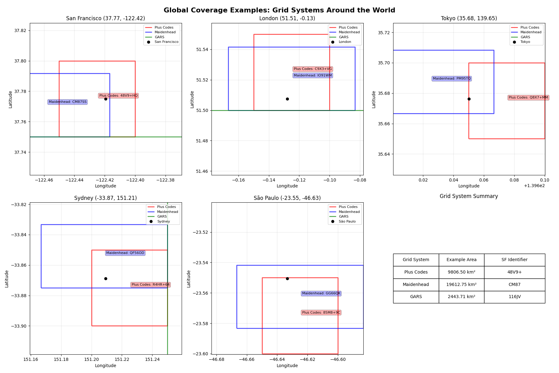
=== Creating Global Coverage Examples ===
Global coverage plots saved as 'global_coverage.png'
============================================================
New Grids Example completed successfully!
Generated visualization files:
- new_grids_comparison.png
- precision_evolution.png
- global_coverage.png
============================================================
import geopandas as gpd
import matplotlib.pyplot as plt
from shapely.geometry import Point

from m3s import GARSGrid, MaidenheadGrid, PlusCodeGrid


def main():
    """Demonstrate the new grid systems."""
    # Test coordinates (San Francisco)
    lat, lon = 37.7749, -122.4194
    print(f"Testing coordinates: {lat}, {lon} (San Francisco)")
    print("=" * 60)

    # Plus codes (Open Location Code)
    print("\n1. Plus codes (Open Location Code)")
    print("-" * 40)

    pluscode_grid = PlusCodeGrid(precision=4)
    pluscode_cell = pluscode_grid.get_cell_from_point(lat, lon)

    print(f"Plus code: {pluscode_cell.identifier}")
    print(f"Cell area: {pluscode_cell.area_km2:.4f} km²")
    print(f"Precision: {pluscode_cell.precision}")

    # Get neighbors
    neighbors = pluscode_grid.get_neighbors(pluscode_cell)
    print(f"Number of neighbors: {len(neighbors)}")

    # Maidenhead locator system
    print("\n2. Maidenhead Locator System")
    print("-" * 40)

    maidenhead_grid = MaidenheadGrid(precision=3)
    maidenhead_cell = maidenhead_grid.get_cell_from_point(lat, lon)

    print(f"Maidenhead locator: {maidenhead_cell.identifier}")
    print(f"Cell area: {maidenhead_cell.area_km2:.4f} km²")
    print(f"Precision: {maidenhead_cell.precision}")

    # Get neighbors
    neighbors = maidenhead_grid.get_neighbors(maidenhead_cell)
    print(f"Number of neighbors: {len(neighbors)}")

    # GARS (Global Area Reference System)
    print("\n3. GARS (Global Area Reference System)")
    print("-" * 40)

    gars_grid = GARSGrid(precision=2)
    gars_cell = gars_grid.get_cell_from_point(lat, lon)

    print(f"GARS identifier: {gars_cell.identifier}")
    print(f"Cell area: {gars_cell.area_km2:.4f} km²")
    print(f"Precision: {gars_cell.precision}")

    # Get neighbors
    neighbors = gars_grid.get_neighbors(gars_cell)
    print(f"Number of neighbors: {len(neighbors)}")

    # Demonstrate bbox functionality
    print("\n4. Bounding Box Queries")
    print("-" * 40)

    # Small bounding box around the test point
    min_lat, min_lon = lat - 0.1, lon - 0.1
    max_lat, max_lon = lat + 0.1, lon + 0.1

    print(
        f"Bounding box: ({min_lat:.2f}, {min_lon:.2f}) to ({max_lat:.2f}, {max_lon:.2f})"
    )

    # Get cells in bbox for each grid system
    pluscode_cells = pluscode_grid.get_cells_in_bbox(min_lat, min_lon, max_lat, max_lon)
    maidenhead_cells = maidenhead_grid.get_cells_in_bbox(
        min_lat, min_lon, max_lat, max_lon
    )
    gars_cells = gars_grid.get_cells_in_bbox(min_lat, min_lon, max_lat, max_lon)

    print(f"Plus codes cells in bbox: {len(pluscode_cells)}")
    print(f"Maidenhead cells in bbox: {len(maidenhead_cells)}")
    print(f"GARS cells in bbox: {len(gars_cells)}")

    # Demonstrate different precisions
    print("\n5. Precision Comparison")
    print("-" * 40)

    print("Plus codes:")
    for precision in range(1, 5):
        grid = PlusCodeGrid(precision=precision)
        cell = grid.get_cell_from_point(lat, lon)
        print(
            f"  Precision {precision}: {cell.identifier} (area: {cell.area_km2:.4f} km²)"
        )

    print("\nMaidenhead:")
    for precision in range(1, 5):
        grid = MaidenheadGrid(precision=precision)
        cell = grid.get_cell_from_point(lat, lon)
        print(
            f"  Precision {precision}: {cell.identifier} (area: {cell.area_km2:.4f} km²)"
        )

    print("\nGARS:")
    for precision in range(1, 4):
        grid = GARSGrid(precision=precision)
        cell = grid.get_cell_from_point(lat, lon)
        print(
            f"  Precision {precision}: {cell.identifier} (area: {cell.area_km2:.4f} km²)"
        )

    # GeoDataFrame integration example
    print("\n6. GeoDataFrame Integration")
    print("-" * 40)

    # Create a simple GeoDataFrame with a point
    gdf = gpd.GeoDataFrame(
        {"name": ["San Francisco"], "geometry": [Point(lon, lat)]}, crs="EPSG:4326"
    )

    # Intersect with different grid systems
    pluscode_result = pluscode_grid.intersects(gdf)
    maidenhead_result = maidenhead_grid.intersects(gdf)
    gars_result = gars_grid.intersects(gdf)

    print(f"Plus codes intersect result: {len(pluscode_result)} cells")
    if len(pluscode_result) > 0:
        print(f"  Cell ID: {pluscode_result.iloc[0]['cell_id']}")

    print(f"Maidenhead intersect result: {len(maidenhead_result)} cells")
    if len(maidenhead_result) > 0:
        print(f"  Cell ID: {maidenhead_result.iloc[0]['cell_id']}")

    print(f"GARS intersect result: {len(gars_result)} cells")
    if len(gars_result) > 0:
        print(f"  Cell ID: {gars_result.iloc[0]['cell_id']}")


def plot_grid_systems_comparison():
    """Create comprehensive plots comparing the new grid systems."""
    print("\n=== Creating Grid Systems Visualization ===")

    # Test coordinates (San Francisco)
    center_lat, center_lon = 37.7749, -122.4194

    # Define visualization area around San Francisco
    offset = 0.05  # Larger area for better visualization
    bounds = (
        center_lon - offset,
        center_lat - offset,
        center_lon + offset,
        center_lat + offset,
    )

    # Create grid instances with different precisions for visualization
    grids = {
        "Plus Codes": PlusCodeGrid(precision=3),
        "Maidenhead": MaidenheadGrid(precision=3),
        "GARS": GARSGrid(precision=2),
    }

    # Create figure with subplots
    fig, axes = plt.subplots(2, 2, figsize=(16, 12))
    fig.suptitle(
        "New Grid Systems in M3S: Plus Codes, Maidenhead, and GARS",
        fontsize=16,
        fontweight="bold",
    )

    # Plot 1: Grid systems overlay comparison
    ax1 = axes[0, 0]
    ax1.set_title("Grid Systems Comparison (San Francisco Area)")
    ax1.set_xlabel("Longitude")
    ax1.set_ylabel("Latitude")

    colors = ["red", "blue", "green"]
    alphas = [0.6, 0.4, 0.3]

    # Plot each grid system
    for i, (name, grid) in enumerate(grids.items()):
        try:
            cells = grid.get_cells_in_bbox(*bounds)
            if cells:
                # Create GeoDataFrame for plotting
                cell_data = []
                for cell in cells[:25]:  # Limit for visibility
                    cell_data.append({"geometry": cell.polygon, "system": name})

                if cell_data:
                    gdf = gpd.GeoDataFrame(cell_data)
                    gdf.boundary.plot(
                        ax=ax1,
                        color=colors[i],
                        alpha=alphas[i],
                        linewidth=1.5,
                        label=name,
                    )
        except Exception as e:
            print(f"Warning: Could not plot {name}: {e}")

    # Add center point
    ax1.plot(center_lon, center_lat, "ko", markersize=8, label="San Francisco")
    ax1.legend()
    ax1.set_xlim(bounds[0], bounds[2])
    ax1.set_ylim(bounds[1], bounds[3])
    ax1.grid(True, alpha=0.3)

    # Plot 2: Cell area comparison across precisions
    ax2 = axes[0, 1]
    ax2.set_title("Cell Areas by Precision Level")
    ax2.set_xlabel("Precision Level")
    ax2.set_ylabel("Cell Area (km²)")
    ax2.set_yscale("log")

    # Calculate areas for different precisions
    precision_ranges = {
        "Plus Codes": range(1, 6),
        "Maidenhead": range(1, 5),
        "GARS": range(1, 4),
    }
    grid_classes = {
        "Plus Codes": PlusCodeGrid,
        "Maidenhead": MaidenheadGrid,
        "GARS": GARSGrid,
    }

    for i, (name, precisions) in enumerate(precision_ranges.items()):
        areas = []
        precision_levels = []

        for precision in precisions:
            try:
                grid = grid_classes[name](precision=precision)
                cell = grid.get_cell_from_point(center_lat, center_lon)
                areas.append(cell.area_km2)
                precision_levels.append(precision)
            except Exception as e:
                print(
                    f"Warning: Could not get area for {name} precision {precision}: {e}"
                )
                continue

        if areas:
            ax2.plot(
                precision_levels,
                areas,
                "o-",
                color=colors[i],
                linewidth=2,
                markersize=6,
                label=name,
            )

    ax2.legend()
    ax2.grid(True, alpha=0.3)

    # Plot 3: Grid density comparison (cells per unit area)
    ax3 = axes[1, 0]
    ax3.set_title("Grid Density Comparison")
    ax3.set_xlabel("Grid System")
    ax3.set_ylabel("Number of Cells in Test Area")

    cell_counts = []
    grid_names = []

    for name, grid in grids.items():
        try:
            cells = grid.get_cells_in_bbox(*bounds)
            cell_counts.append(len(cells))
            grid_names.append(name)
        except Exception as e:
            print(f"Warning: Could not count cells for {name}: {e}")
            continue

    if cell_counts:
        bars = ax3.bar(
            grid_names, cell_counts, color=colors[: len(cell_counts)], alpha=0.7
        )
        ax3.set_ylim(0, max(cell_counts) * 1.1)

        # Add value labels on bars
        for bar, count in zip(bars, cell_counts):
            ax3.text(
                bar.get_x() + bar.get_width() / 2,
                bar.get_height() + max(cell_counts) * 0.01,
                str(count),
                ha="center",
                va="bottom",
                fontweight="bold",
            )

    ax3.grid(True, alpha=0.3)

    # Plot 4: Individual grid system details
    ax4 = axes[1, 1]
    ax4.set_title("Grid System Characteristics")
    ax4.axis("off")

    # Create text summary of grid characteristics
    characteristics = {
        "Plus Codes": {
            "Full Name": "Open Location Code",
            "Developed by": "Google",
            "Cell Shape": "Rectangular",
            "Precision Range": "1-11",
            "Use Case": "Address replacement",
        },
        "Maidenhead": {
            "Full Name": "Maidenhead Locator System",
            "Developed by": "Amateur Radio",
            "Cell Shape": "Rectangular",
            "Precision Range": "1-8",
            "Use Case": "Ham radio communication",
        },
        "GARS": {
            "Full Name": "Global Area Reference System",
            "Developed by": "NGA (formerly NIMA)",
            "Cell Shape": "Rectangular",
            "Precision Range": "1-3",
            "Use Case": "Military/government mapping",
        },
    }

    y_pos = 0.9
    for name, details in characteristics.items():
        ax4.text(
            0.05,
            y_pos,
            f"{name}:",
            fontsize=12,
            fontweight="bold",
            transform=ax4.transAxes,
            color=colors[list(characteristics.keys()).index(name)],
        )
        y_pos -= 0.06

        for key, value in details.items():
            ax4.text(
                0.1, y_pos, f"{key}: {value}", fontsize=10, transform=ax4.transAxes
            )
            y_pos -= 0.05
        y_pos -= 0.03

    plt.tight_layout()
    plt.savefig("new_grids_comparison.png", dpi=150, bbox_inches="tight")
    print("Grid comparison plots saved as 'new_grids_comparison.png'")
    plt.show()


def plot_precision_evolution():
    """Create plots showing how grid precision affects cell size and coverage."""
    print("\n=== Creating Precision Evolution Plots ===")

    # Test coordinates
    center_lat, center_lon = 37.7749, -122.4194

    fig, axes = plt.subplots(1, 3, figsize=(18, 6))
    fig.suptitle(
        "Grid Precision Evolution: Cell Size and Coverage",
        fontsize=16,
        fontweight="bold",
    )

    colors = ["red", "blue", "green"]
    grid_systems = [
        ("Plus Codes", PlusCodeGrid, range(2, 6)),
        ("Maidenhead", MaidenheadGrid, range(2, 5)),
        ("GARS", GARSGrid, range(1, 4)),
    ]

    for idx, (name, grid_class, precision_range) in enumerate(grid_systems):
        ax = axes[idx]
        ax.set_title(f"{name} Precision Evolution")
        ax.set_xlabel("Longitude")
        ax.set_ylabel("Latitude")

        # Plot different precision levels
        for precision in precision_range:
            try:
                grid = grid_class(precision=precision)
                cell = grid.get_cell_from_point(center_lat, center_lon)

                # Create GeoDataFrame for this cell
                gdf = gpd.GeoDataFrame([{"geometry": cell.polygon}])

                # Plot with different alpha based on precision
                alpha = 0.3 + (precision - min(precision_range)) * 0.2
                gdf.boundary.plot(
                    ax=ax,
                    color=colors[idx],
                    alpha=alpha,
                    linewidth=2,
                    label=f"Precision {precision}",
                )

            except Exception as e:
                print(f"Warning: Could not plot {name} precision {precision}: {e}")
                continue

        # Add center point
        ax.plot(center_lon, center_lat, "ko", markersize=6)
        ax.legend()
        ax.grid(True, alpha=0.3)

        # Set reasonable bounds around the center point
        offset = 0.02
        ax.set_xlim(center_lon - offset, center_lon + offset)
        ax.set_ylim(center_lat - offset, center_lat + offset)

    plt.tight_layout()
    plt.savefig("precision_evolution.png", dpi=150, bbox_inches="tight")
    print("Precision evolution plots saved as 'precision_evolution.png'")
    plt.show()


def plot_global_coverage():
    """Create a plot showing global coverage examples of the grid systems."""
    print("\n=== Creating Global Coverage Examples ===")

    # Define interesting global locations
    locations = {
        "San Francisco": (37.7749, -122.4194),
        "London": (51.5074, -0.1278),
        "Tokyo": (35.6762, 139.6503),
        "Sydney": (-33.8688, 151.2093),
        "São Paulo": (-23.5505, -46.6333),
    }

    fig, axes = plt.subplots(2, 3, figsize=(18, 12))
    fig.suptitle(
        "Global Coverage Examples: Grid Systems Around the World",
        fontsize=16,
        fontweight="bold",
    )

    # Flatten axes for easier iteration
    axes_flat = axes.flatten()

    # Create one subplot per location
    for idx, (city, (lat, lon)) in enumerate(locations.items()):
        if idx >= len(axes_flat):
            break

        ax = axes_flat[idx]
        ax.set_title(f"{city} ({lat:.2f}, {lon:.2f})")
        ax.set_xlabel("Longitude")
        ax.set_ylabel("Latitude")

        colors = ["red", "blue", "green"]
        grids = [
            ("Plus Codes", PlusCodeGrid(precision=3)),
            ("Maidenhead", MaidenheadGrid(precision=3)),
            ("GARS", GARSGrid(precision=2)),
        ]

        offset = 0.05
        bounds = (lon - offset, lat - offset, lon + offset, lat + offset)

        for i, (name, grid) in enumerate(grids):
            try:
                # Get the cell containing this location
                cell = grid.get_cell_from_point(lat, lon)
                gdf = gpd.GeoDataFrame([{"geometry": cell.polygon}])
                gdf.boundary.plot(
                    ax=ax, color=colors[i], alpha=0.7, linewidth=2, label=name
                )

                # Add cell identifier as text
                centroid = cell.polygon.centroid
                ax.annotate(
                    f"{name}: {cell.identifier}",
                    xy=(centroid.x, centroid.y),
                    xytext=(5, 5),
                    textcoords="offset points",
                    fontsize=8,
                    bbox={"boxstyle": "round,pad=0.3", "fc": colors[i], "alpha": 0.3},
                )

            except Exception as e:
                print(f"Warning: Could not plot {name} for {city}: {e}")
                continue

        # Add location point
        ax.plot(lon, lat, "ko", markersize=6, label=city)
        ax.legend(fontsize=8)
        ax.grid(True, alpha=0.3)
        ax.set_xlim(bounds[0], bounds[2])
        ax.set_ylim(bounds[1], bounds[3])

    # Use the last subplot for summary statistics
    if len(locations) < len(axes_flat):
        ax_summary = axes_flat[-1]
        ax_summary.set_title("Grid System Summary")
        ax_summary.axis("off")

        # Create summary table
        summary_data = []
        for name, grid_class in [
            ("Plus Codes", PlusCodeGrid),
            ("Maidenhead", MaidenheadGrid),
            ("GARS", GARSGrid),
        ]:
            try:
                grid = grid_class(precision=2 if name != "GARS" else 1)
                cell = grid.get_cell_from_point(37.7749, -122.4194)  # SF coordinates
                summary_data.append([name, f"{cell.area_km2:.2f} km²", cell.identifier])
            except Exception:
                summary_data.append([name, "Error", "N/A"])

        # Create table
        table = ax_summary.table(
            cellText=summary_data,
            colLabels=["Grid System", "Example Area", "SF Identifier"],
            cellLoc="center",
            loc="center",
            colWidths=[0.3, 0.3, 0.4],
        )
        table.auto_set_font_size(False)
        table.set_fontsize(10)
        table.scale(1, 2)

    plt.tight_layout()
    plt.savefig("global_coverage.png", dpi=150, bbox_inches="tight")
    print("Global coverage plots saved as 'global_coverage.png'")
    plt.show()


if __name__ == "__main__":
    main()

    # Create comprehensive visualizations
    plot_grid_systems_comparison()
    plot_precision_evolution()
    plot_global_coverage()

    print("\n" + "=" * 60)
    print("New Grids Example completed successfully!")
    print("Generated visualization files:")
    print("- new_grids_comparison.png")
    print("- precision_evolution.png")
    print("- global_coverage.png")
    print("=" * 60)
Total running time of the script: (0 minutes 9.514 seconds)