Note
Go to the end to download the full example code.
Grid System Enhancements Example.
This example demonstrates the new grid system enhancements in M3S: 1. What3Words integration 2. Grid conversion utilities 3. Grid cell relationship analysis 4. Multi-resolution grid operations
M3S Grid System Enhancements Demo
==================================================
=== What3Words Grid System ===
What3Words cell area: 9e-06 km²
NYC What3Words cell: w3w.wde.we7.w3b
Cell area: 0.000008985 km²
Number of neighbors: 8
Neighbor identifiers: ['w3w.wdd.w96.w79...', 'w3w.w30.w77.w1b...', 'w3w.w07.w28.w10...']
=== Grid Conversion Utilities ===
Available grid systems:
system default_precision default_area_km2
0 geohash 5 4892.000000
1 mgrs 1 100.000000
2 h3 7 5.160000
3 quadkey 12 95.725395
4 s2 10 81.073761
Source Geohash cell: dr5re
Source cell area: 18.11 km²
Conversions:
H3: 872a1072effffff
Quadkey: 032010110123
What3Words: w3w.w15.w07.wbf
Conversion table (Geohash -> H3): 2 mappings
source_system source_id source_precision target_system target_id target_precision conversion_method
0 geohash dr5re 5 h3 872a1072effffff 7 centroid
1 geohash dr5rs 5 h3 872a1072dffffff 7 centroid
=== Grid Cell Relationship Analysis ===
Analyzing relationships for 4 cells
Relationship between first two cells: touches
Adjacent cells to first cell: 3
Adjacency matrix:
dr5rs5 dr5reg dr5rsh dr5reu
dr5rs5 0 1 1 1
dr5reg 1 0 1 1
dr5rsh 1 1 0 1
dr5reu 1 1 1 0
Network connectivity: 1.000
=== Multi-Resolution Grid Operations ===
Multi-resolution grid with 4 levels
Resolution levels:
level precision area_km2
0 0 4 39135.0
1 1 5 4892.0
2 2 6 1223.0
3 3 7 153.0
Hierarchical cells for NYC:
Precision 4: dr5r (579.69 km²)
Precision 5: dr5re (18.11 km²)
Precision 6: dr5reg (0.57 km²)
Precision 7: dr5regw (0.02 km²)
Scale transitions:
from_precision to_precision subdivision_ratio
0 4 5 2.0
1 5 6 15.0
2 6 7 23.0
Adaptive grid contains 120 cells
Cells by precision level:
Precision 5: 120 cells
=== Combined Visualization Example ===
/home/runner/work/m3s/m3s/examples/grid_enhancements_example.py:178: DeprecationWarning: The 'resolution' parameter is deprecated. Use 'precision' instead.
h3_grid = H3Grid(resolution=9)
Geohash cells: 32
H3 cells: 59
Converted 5 Geohash cells to 10 H3 cells
Found 15 adjacent cell pairs in sample of 10 cells
Visualization example completed!
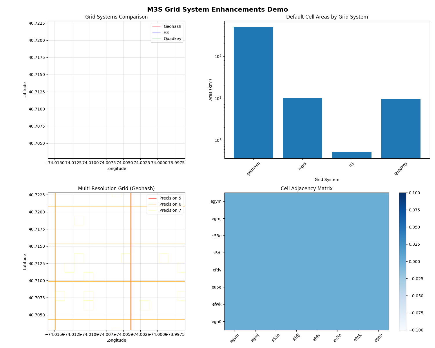
=== Creating Grid System Comparison Plots ===
/home/runner/work/m3s/m3s/examples/grid_enhancements_example.py:237: DeprecationWarning: The 'resolution' parameter is deprecated. Use 'precision' instead.
"H3": H3Grid(resolution=9),
/home/runner/work/m3s/m3s/examples/grid_enhancements_example.py:238: DeprecationWarning: The 'level' parameter is deprecated. Use 'precision' instead.
"Quadkey": QuadkeyGrid(level=15),
Plots saved as 'grid_enhancements_demo.png'
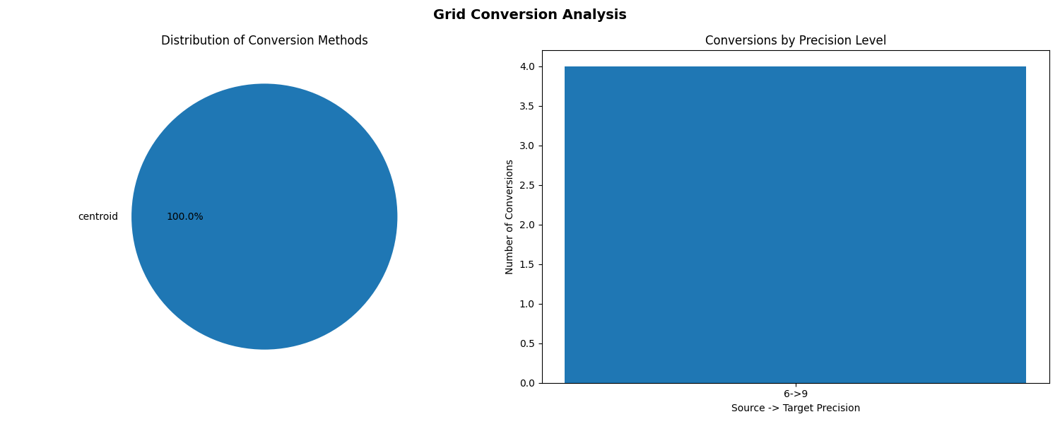
=== Creating Grid Conversion Analysis Plots ===
Conversion analysis plots saved as 'conversion_analysis.png'
All demonstrations completed successfully!
Key features demonstrated:
✓ What3Words grid integration with 3m precision
✓ Grid conversion between different systems
✓ Spatial relationship analysis (containment, adjacency)
✓ Multi-resolution grid operations with adaptive selection
✓ Combined workflows using multiple enhancement features
✓ Comprehensive visualizations and plots
import geopandas as gpd
import matplotlib.pyplot as plt
import numpy as np
from shapely.geometry import Point

from m3s import (
    GeohashGrid,
    H3Grid,
    QuadkeyGrid,
    What3WordsGrid,
    analyze_relationship,
    convert_cell,
    create_adaptive_grid,
    create_adjacency_matrix,
    create_conversion_table,
    create_multiresolution_grid,
    find_adjacent_cells,
    list_grid_systems,
)


def demonstrate_what3words():
    """Demonstrate What3Words grid integration."""
    print("=== What3Words Grid System ===")

    # Create What3Words grid
    w3w_grid = What3WordsGrid()
    print(f"What3Words cell area: {w3w_grid.area_km2} km²")

    # Get cell for NYC coordinates
    nyc_cell = w3w_grid.get_cell_from_point(40.7128, -74.0060)
    print(f"NYC What3Words cell: {nyc_cell.identifier}")
    print(f"Cell area: {nyc_cell.area_km2:.9f} km²")

    # Find neighbors
    neighbors = w3w_grid.get_neighbors(nyc_cell)
    print(f"Number of neighbors: {len(neighbors)}")
    print("Neighbor identifiers:", [n.identifier[:20] + "..." for n in neighbors[:3]])

    print()


def demonstrate_grid_conversion():
    """Demonstrate grid conversion utilities."""
    print("=== Grid Conversion Utilities ===")

    # List available grid systems
    systems_info = list_grid_systems()
    print("Available grid systems:")
    print(systems_info[["system", "default_precision", "default_area_km2"]].head())
    print()

    # Create source cell (Geohash)
    geohash_grid = GeohashGrid(precision=5)
    source_cell = geohash_grid.get_cell_from_point(40.7128, -74.0060)
    print(f"Source Geohash cell: {source_cell.identifier}")
    print(f"Source cell area: {source_cell.area_km2:.2f} km²")

    # Convert to different systems
    h3_cell = convert_cell(source_cell, "h3", method="centroid")
    quadkey_cell = convert_cell(source_cell, "quadkey", method="centroid")
    w3w_cell = convert_cell(source_cell, "what3words", method="centroid")

    print("\nConversions:")
    print(f"  H3: {h3_cell.identifier}")
    print(f"  Quadkey: {quadkey_cell.identifier}")
    print(f"  What3Words: {w3w_cell.identifier}")

    # Create conversion table for small area
    bounds = (-74.01, 40.71, -74.00, 40.72)
    conversion_table = create_conversion_table(
        "geohash", "h3", bounds, source_precision=5, target_precision=7
    )
    print(f"\nConversion table (Geohash -> H3): {len(conversion_table)} mappings")
    print(conversion_table.head())

    print()


def demonstrate_relationship_analysis():
    """Demonstrate grid cell relationship analysis."""
    print("=== Grid Cell Relationship Analysis ===")

    # Create test cells
    geohash_grid = GeohashGrid(precision=6)

    # Get cells in a small region
    cells = geohash_grid.get_cells_in_bbox(40.71, -74.01, 40.72, -74.00)
    print(f"Analyzing relationships for {len(cells)} cells")

    if len(cells) >= 2:
        # Analyze relationship between first two cells
        relationship = analyze_relationship(cells[0], cells[1])
        print(f"Relationship between first two cells: {relationship.value}")

        # Find adjacent cells to the first cell
        adjacent = find_adjacent_cells(cells[0], cells[1:])
        print(f"Adjacent cells to first cell: {len(adjacent)}")

        # Create adjacency matrix (limit to first 5 cells for readability)
        sample_cells = cells[: min(5, len(cells))]
        adj_matrix = create_adjacency_matrix(sample_cells)
        print("\nAdjacency matrix:")
        print(adj_matrix)

        # Calculate connectivity
        total_connections = adj_matrix.sum().sum()
        max_connections = len(sample_cells) * (len(sample_cells) - 1)
        connectivity = total_connections / max_connections if max_connections > 0 else 0
        print(f"Network connectivity: {connectivity:.3f}")

    print()


def demonstrate_multiresolution():
    """Demonstrate multi-resolution grid operations."""
    print("=== Multi-Resolution Grid Operations ===")

    # Create multi-resolution grid with Geohash
    base_grid = GeohashGrid(precision=5)
    resolution_levels = [4, 5, 6, 7]  # Coarse to fine

    multi_grid = create_multiresolution_grid(base_grid, resolution_levels)
    print(f"Multi-resolution grid with {len(resolution_levels)} levels")

    # Get resolution statistics
    stats = multi_grid.get_resolution_statistics()
    print("Resolution levels:")
    print(stats[["level", "precision", "area_km2"]])

    # Get hierarchical cells for NYC
    nyc_point = Point(-74.0060, 40.7128)
    hierarchical_cells = multi_grid.get_hierarchical_cells(nyc_point)

    print("\nHierarchical cells for NYC:")
    for precision, cell in hierarchical_cells.items():
        print(f"  Precision {precision}: {cell.identifier} ({cell.area_km2:.2f} km²)")

    # Populate region and analyze scale transitions
    bounds = (-74.02, 40.70, -73.98, 40.73)
    multi_grid.populate_region(bounds)

    transitions = multi_grid.analyze_scale_transitions(bounds)
    print("\nScale transitions:")
    print(transitions[["from_precision", "to_precision", "subdivision_ratio"]])

    # Create adaptive grid
    adaptive_gdf = create_adaptive_grid(base_grid, bounds, resolution_levels)
    print(f"\nAdaptive grid contains {len(adaptive_gdf)} cells")
    if len(adaptive_gdf) > 0:
        precision_counts = adaptive_gdf["precision"].value_counts().sort_index()
        print("Cells by precision level:")
        for precision, count in precision_counts.items():
            print(f"  Precision {precision}: {count} cells")

    print()


def create_visualization_example():
    """Create a visualization example combining multiple enhancements."""
    print("=== Combined Visualization Example ===")

    # Define NYC area
    bounds = (-74.02, 40.70, -73.98, 40.73)

    # Create different grid systems
    geohash_grid = GeohashGrid(precision=6)
    h3_grid = H3Grid(resolution=9)

    # Get cells from each system
    geohash_cells = geohash_grid.get_cells_in_bbox(*bounds)
    h3_cells = h3_grid.get_cells_in_bbox(*bounds)

    print(f"Geohash cells: {len(geohash_cells)}")
    print(f"H3 cells: {len(h3_cells)}")

    # Convert some geohash cells to H3
    if geohash_cells:
        converted_cells = []
        for cell in geohash_cells[:5]:  # Convert first 5
            h3_converted = convert_cell(cell, "h3", method="overlap")
            if isinstance(h3_converted, list):
                converted_cells.extend(h3_converted)
            else:
                converted_cells.append(h3_converted)

        print(
            f"Converted {len(geohash_cells[:5])} Geohash cells to {len(converted_cells)} H3 cells"
        )

    # Analyze relationships within H3 cells
    if len(h3_cells) > 1:
        adjacent_pairs = 0
        sample_cells = h3_cells[: min(10, len(h3_cells))]

        for i, cell1 in enumerate(sample_cells):
            for _j, cell2 in enumerate(sample_cells[i + 1 :], i + 1):
                rel = analyze_relationship(cell1, cell2)
                if rel.value in ["touches", "adjacent"]:
                    adjacent_pairs += 1

        print(
            f"Found {adjacent_pairs} adjacent cell pairs in sample of {len(sample_cells)} cells"
        )

    print("Visualization example completed!")
    print()


def plot_grid_comparison():
    """Create plots comparing different grid systems."""
    print("=== Creating Grid System Comparison Plots ===")

    # Define a small area for visualization
    center_lat, center_lon = 40.7128, -74.0060
    offset = 0.01  # Small area around NYC
    bounds = (
        center_lon - offset,
        center_lat - offset,
        center_lon + offset,
        center_lat + offset,
    )

    # Create different grid systems with similar cell sizes
    grids = {
        "Geohash": GeohashGrid(precision=7),
        "H3": H3Grid(resolution=9),
        "Quadkey": QuadkeyGrid(level=15),
    }

    # Create subplot figure
    fig, axes = plt.subplots(2, 2, figsize=(15, 12))
    fig.suptitle("M3S Grid System Enhancements Demo", fontsize=16, fontweight="bold")

    # Plot 1: Grid system comparison
    ax1 = axes[0, 0]
    ax1.set_title("Grid Systems Comparison")
    ax1.set_xlabel("Longitude")
    ax1.set_ylabel("Latitude")

    colors = ["red", "blue", "green"]
    alphas = [0.3, 0.3, 0.3]

    for i, (name, grid) in enumerate(grids.items()):
        cells = grid.get_cells_in_bbox(*bounds)
        if cells:
            # Create GeoDataFrame for plotting
            cell_data = []
            for cell in cells[:20]:  # Limit for visibility
                cell_data.append({"geometry": cell.polygon, "system": name})

            if cell_data:
                gdf = gpd.GeoDataFrame(cell_data)
                gdf.boundary.plot(
                    ax=ax1, color=colors[i], alpha=alphas[i], linewidth=1, label=name
                )

    ax1.legend()
    ax1.set_xlim(bounds[0], bounds[2])
    ax1.set_ylim(bounds[1], bounds[3])
    ax1.grid(True, alpha=0.3)

    # Plot 2: Cell area comparison
    ax2 = axes[0, 1]
    systems_info = list_grid_systems()
    if len(systems_info) > 0:
        # Filter to systems we can actually use
        plot_systems = systems_info[
            systems_info["system"].isin(["geohash", "h3", "quadkey", "mgrs"])
        ].copy()

        if len(plot_systems) > 0:
            ax2.bar(plot_systems["system"], plot_systems["default_area_km2"])
            ax2.set_title("Default Cell Areas by Grid System")
            ax2.set_xlabel("Grid System")
            ax2.set_ylabel("Area (km²)")
            ax2.set_yscale("log")
            plt.setp(ax2.get_xticklabels(), rotation=45)

    # Plot 3: Multi-resolution demonstration
    ax3 = axes[1, 0]
    ax3.set_title("Multi-Resolution Grid (Geohash)")
    ax3.set_xlabel("Longitude")
    ax3.set_ylabel("Latitude")

    # Create multi-resolution grid
    base_grid = GeohashGrid(precision=5)
    multi_grid = create_multiresolution_grid(base_grid, [5, 6, 7])

    colors_multi = ["red", "orange", "yellow"]
    alphas_multi = [0.6, 0.4, 0.2]

    level_cells = multi_grid.populate_region(bounds)
    for i, (precision, cells) in enumerate(level_cells.items()):
        if cells:
            cell_data = []
            for cell in cells[:15]:  # Limit for visibility
                cell_data.append({"geometry": cell.polygon, "precision": precision})

            if cell_data:
                gdf = gpd.GeoDataFrame(cell_data)
                gdf.boundary.plot(
                    ax=ax3,
                    color=colors_multi[i],
                    alpha=alphas_multi[i],
                    linewidth=2 - i * 0.5,
                    label=f"Precision {precision}",
                )

    ax3.legend()
    ax3.set_xlim(bounds[0], bounds[2])
    ax3.set_ylim(bounds[1], bounds[3])
    ax3.grid(True, alpha=0.3)

    # Plot 4: Adjacency matrix heatmap
    ax4 = axes[1, 1]
    ax4.set_title("Cell Adjacency Matrix")

    # Get a small sample of cells for adjacency analysis
    sample_grid = GeohashGrid(precision=8)
    sample_cells = sample_grid.get_cells_in_bbox(
        center_lat - 0.005, center_lon - 0.005, center_lat + 0.005, center_lon + 0.005
    )

    if len(sample_cells) > 1:
        # Limit to reasonable number for visualization
        sample_cells = sample_cells[: min(8, len(sample_cells))]
        adj_matrix = create_adjacency_matrix(sample_cells)

        # Convert to numpy array for plotting
        matrix_values = adj_matrix.values

        im = ax4.imshow(matrix_values, cmap="Blues", aspect="auto")
        ax4.set_xticks(range(len(sample_cells)))
        ax4.set_yticks(range(len(sample_cells)))
        ax4.set_xticklabels(
            [cell.identifier[-4:] for cell in sample_cells], rotation=45
        )
        ax4.set_yticklabels([cell.identifier[-4:] for cell in sample_cells])

        # Add colorbar
        plt.colorbar(im, ax=ax4)
    else:
        ax4.text(
            0.5,
            0.5,
            "Insufficient cells\nfor adjacency analysis",
            ha="center",
            va="center",
            transform=ax4.transAxes,
        )

    plt.tight_layout()
    plt.savefig("grid_enhancements_demo.png", dpi=150, bbox_inches="tight")
    print("Plots saved as 'grid_enhancements_demo.png'")
    plt.show()
    print()


def plot_conversion_analysis():
    """Create plots showing grid conversion analysis."""
    print("=== Creating Grid Conversion Analysis Plots ===")

    # Define analysis area
    bounds = (-74.01, 40.71, -74.00, 40.72)

    # Create conversion table
    try:
        conversion_table = create_conversion_table(
            "geohash", "h3", bounds, source_precision=6, target_precision=9
        )

        if len(conversion_table) > 0:
            fig, (ax1, ax2) = plt.subplots(1, 2, figsize=(15, 6))
            fig.suptitle("Grid Conversion Analysis", fontsize=14, fontweight="bold")

            # Plot 1: Conversion method distribution
            method_counts = conversion_table["conversion_method"].value_counts()
            ax1.pie(method_counts.values, labels=method_counts.index, autopct="%1.1f%%")
            ax1.set_title("Distribution of Conversion Methods")

            # Plot 2: Precision level comparison
            precision_data = (
                conversion_table.groupby(["source_precision", "target_precision"])
                .size()
                .reset_index(name="count")
            )

            if len(precision_data) > 0:
                x_pos = np.arange(len(precision_data))
                ax2.bar(x_pos, precision_data["count"])
                ax2.set_title("Conversions by Precision Level")
                ax2.set_xlabel("Source -> Target Precision")
                ax2.set_ylabel("Number of Conversions")

                labels = [
                    f"{row['source_precision']}->{row['target_precision']}"
                    for _, row in precision_data.iterrows()
                ]
                ax2.set_xticks(x_pos)
                ax2.set_xticklabels(labels)

            plt.tight_layout()
            plt.savefig("conversion_analysis.png", dpi=150, bbox_inches="tight")
            print("Conversion analysis plots saved as 'conversion_analysis.png'")
            plt.show()
        else:
            print("No conversion data available for plotting")

    except Exception as e:
        print(f"Could not create conversion analysis plots: {e}")

    print()


def main():
    """Main function to run all demonstrations."""
    print("M3S Grid System Enhancements Demo")
    print("=" * 50)
    print()

    demonstrate_what3words()
    demonstrate_grid_conversion()
    demonstrate_relationship_analysis()
    demonstrate_multiresolution()
    create_visualization_example()

    # Create visualizations
    plot_grid_comparison()
    plot_conversion_analysis()

    print("All demonstrations completed successfully!")
    print("\nKey features demonstrated:")
    print("✓ What3Words grid integration with 3m precision")
    print("✓ Grid conversion between different systems")
    print("✓ Spatial relationship analysis (containment, adjacency)")
    print("✓ Multi-resolution grid operations with adaptive selection")
    print("✓ Combined workflows using multiple enhancement features")
    print("✓ Comprehensive visualizations and plots")


if __name__ == "__main__":
    main()
Total running time of the script: (0 minutes 5.005 seconds)