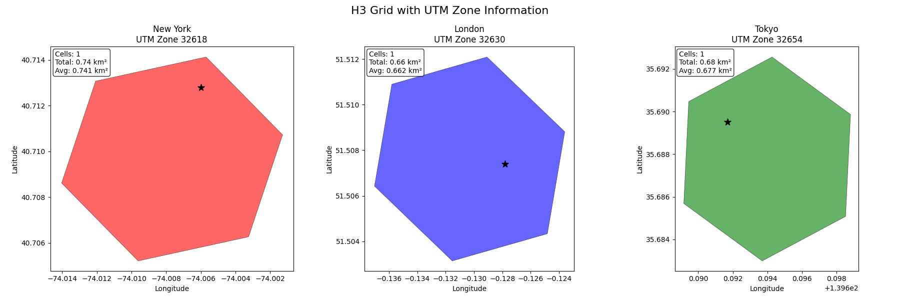
Reproject grid using UTM zone information and visualize.

This example demonstrates how to use the UTM zone information provided by the grid systems to reproject the results and visualize area differences.

Original GeoDataFrame (WGS84):
       city country
0  New York     USA
1    London      UK
2     Tokyo   Japan
CRS: EPSG:4326

Generating H3 grid (resolution 8)...
/home/runner/work/m3s/m3s/examples/utm_reprojection_example.py:32: DeprecationWarning: The 'resolution' parameter is deprecated. Use 'precision' instead.
  h3_grid = H3Grid(resolution=8)
Generated 3 H3 cells
UTM zones found: [np.int64(32618), np.int64(32630), np.int64(32654)]

Reprojecting to UTM zones for accurate area calculation...
UTM Zone 32618: New York
  Total area: 0.74 km²
UTM Zone 32630: London
  Total area: 0.66 km²
UTM Zone 32654: Tokyo
  Total area: 0.68 km²

Area Analysis:
New York (UTM 32618):
  Cells: 1
  Total area: 0.741 km²
  Average cell area: 0.741 km²

London (UTM 32630):
  Cells: 1
  Total area: 0.662 km²
  Average cell area: 0.662 km²

Tokyo (UTM 32654):
  Cells: 1
  Total area: 0.677 km²
  Average cell area: 0.677 km²

Key insight: Each city uses its optimal UTM zone for accurate area calculations

import geopandas as gpd
import matplotlib.pyplot as plt
from shapely.geometry import Point

from m3s import H3Grid

# Create a GeoDataFrame with points across different UTM zones
gdf = gpd.GeoDataFrame(
    {"city": ["New York", "London", "Tokyo"], "country": ["USA", "UK", "Japan"]},
    geometry=[
        Point(-74.0060, 40.7128),  # NYC (UTM 18N)
        Point(-0.1278, 51.5074),  # London (UTM 30N)
        Point(139.6917, 35.6895),  # Tokyo (UTM 54N)
    ],
    crs="EPSG:4326",
)

print("Original GeoDataFrame (WGS84):")
print(gdf[["city", "country"]])
print(f"CRS: {gdf.crs}")

# Generate H3 grid cells
print("\nGenerating H3 grid (resolution 8)...")
h3_grid = H3Grid(resolution=8)
h3_result = h3_grid.intersects(gdf)

print(f"Generated {len(h3_result)} H3 cells")
print("UTM zones found:", sorted(h3_result["utm"].unique()))

# Reproject each group to its UTM zone and calculate areas
print("\nReprojecting to UTM zones for accurate area calculation...")
reprojected_results = []

for utm_zone in h3_result["utm"].unique():
    zone_cells = h3_result[h3_result["utm"] == utm_zone].copy()
    utm_crs = f"EPSG:{utm_zone}"
    zone_cells_utm = zone_cells.to_crs(utm_crs)
    zone_cells_utm["area_m2"] = zone_cells_utm.geometry.area
    zone_cells_utm["area_km2"] = zone_cells_utm["area_m2"] / 1_000_000

    cities_in_zone = zone_cells_utm["city"].unique()
    print(f"UTM Zone {utm_zone}: {', '.join(cities_in_zone)}")
    print(f"  Total area: {zone_cells_utm['area_km2'].sum():.2f} km²")

    reprojected_results.append(zone_cells_utm)

# Convert each UTM result back to WGS84 first, then combine
import pandas as pd

reprojected_wgs84 = []
for utm_result in reprojected_results:
    utm_result_wgs84 = utm_result.to_crs("EPSG:4326")
    reprojected_wgs84.append(utm_result_wgs84)

# Now combine all results (all in WGS84)
all_utm_cells_wgs84 = gpd.GeoDataFrame(pd.concat(reprojected_wgs84, ignore_index=True))

# Create visualization
fig, axes = plt.subplots(1, 3, figsize=(18, 6))
fig.suptitle("H3 Grid with UTM Zone Information", fontsize=16)

# Plot by city
cities = gdf["city"].unique()
colors = ["red", "blue", "green"]

for i, city in enumerate(cities):
    # Filter data for this city
    city_original = gdf[gdf["city"] == city]
    city_grid = all_utm_cells_wgs84[all_utm_cells_wgs84["city"] == city]
    utm_zone = city_grid["utm"].iloc[0]

    # Plot
    axes[i].set_title(f"{city}\nUTM Zone {utm_zone}")

    # Plot grid cells
    city_grid.plot(
        ax=axes[i], alpha=0.6, edgecolor="black", linewidth=0.5, color=colors[i]
    )

    # Plot original point
    city_original.plot(ax=axes[i], color="black", markersize=100, marker="*")

    axes[i].set_xlabel("Longitude")
    axes[i].set_ylabel("Latitude")

    # Add area info as text
    total_area = city_grid["area_km2"].sum()
    avg_area = city_grid["area_km2"].mean()
    cell_count = len(city_grid)

    info_text = (
        f"Cells: {cell_count}\nTotal: {total_area:.2f} km²\nAvg: {avg_area:.3f} km²"
    )
    axes[i].text(
        0.02,
        0.98,
        info_text,
        transform=axes[i].transAxes,
        verticalalignment="top",
        bbox={"boxstyle": "round", "facecolor": "white", "alpha": 0.8},
    )

plt.tight_layout()
plt.show()

# Print area comparison
print("\nArea Analysis:")
for city in cities:
    # Find the city data in the original UTM results
    city_data = None
    for utm_result in reprojected_results:
        if city in utm_result["city"].values:
            city_data = utm_result[utm_result["city"] == city]
            break
    utm_zone = city_data["utm"].iloc[0]
    total_area = city_data["area_km2"].sum()
    avg_area = city_data["area_km2"].mean()
    cell_count = len(city_data)

    print(f"{city} (UTM {utm_zone}):")
    print(f"  Cells: {cell_count}")
    print(f"  Total area: {total_area:.3f} km²")
    print(f"  Average cell area: {avg_area:.3f} km²")
    print()

print("Key insight: Each city uses its optimal UTM zone for accurate area calculations")