Quickstart

The GIS-native M3S API — the default entry point.

It provides:

• Direct access to grid systems via m3s.H3, m3s.Geohash, etc.

• A universal from_geometry() method handling any geometry type

• Auto-precision selection for optimal coverage

• Easy conversions between grid systems

• Convenient collection operations

All coordinate tuples use GIS-native (lon, lat) order.

import geopandas as gpd
import matplotlib.pyplot as plt
from shapely.geometry import Polygon

import m3s

Example 1: Universal from_geometry() - works with any geometry type

The from_geometry() method accepts point tuples, Polygons, GeoDataFrames, and bounding box tuples. Precision is auto-selected for optimal coverage.

# Point tuple (lon, lat) - GIS-native axis order
cell = m3s.Geohash.from_geometry((-74.0060, 40.7128))
print(f"Cell: {cell.id}, Area: {cell.area_km2:.2f} km²")
print(f"Centroid: {cell.centroid}")
print(f"Bounds: {cell.bounds}")

Cell: dr5re, Area: 18.10 km²
Centroid: (-74.02587890625, 40.71533203125)
Bounds: (-74.0478515625, 40.693359375, -74.00390625, 40.7373046875)

Example 2: from_geometry() with Polygon — and see the result

Uses default precision (or specify for optimal coverage). The collection plots directly with matplotlib via .plot().

polygon = Polygon([(-74.1, 40.7), (-73.9, 40.7), (-73.9, 40.8), (-74.1, 40.8)])
cells = m3s.H3.from_geometry(polygon)  # Uses default precision (7)
print(f"Found {len(cells)} H3 cells, total area {cells.total_area_km2:.2f} km²")

ax = cells.plot(edgecolor="white", linewidth=0.8)
gpd.GeoSeries([polygon], crs="EPSG:4326").boundary.plot(ax=ax, color="red")
ax.set_title(f"{len(cells)} H3 cells covering the polygon (red outline)")
plt.tight_layout()

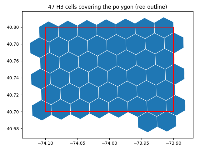
Found 47 H3 cells, total area 243.86 km²

Example 3: Interactive map with explore()

.explore() delegates to GeoPandas/folium and returns a Leaflet map — pan, zoom and hover the cells below.

cells.explore(tooltip="cell_id")

Make this Notebook Trusted to load map: File -> Trust Notebook

Example 4: from_geometry() with GeoDataFrame

gdf = gpd.GeoDataFrame({"geometry": [polygon]}, crs="EPSG:4326")
cells_s2 = m3s.S2.from_geometry(gdf)
print(f"S2 cells from GeoDataFrame: {len(cells_s2)} cells")

S2 cells from GeoDataFrame: 8 cells

Example 5: One area, four grid systems

The same polygon tiled by four grids — same API call each time, different cell shapes and counts.

fig, axes = plt.subplots(2, 2, figsize=(10, 8))
outline = gpd.GeoSeries([polygon], crs="EPSG:4326").boundary
grids = [
    ("H3", m3s.H3),
    ("Geohash", m3s.Geohash),
    ("S2", m3s.S2),
    ("Quadkey", m3s.Quadkey),
]
for ax, (name, grid) in zip(axes.flat, grids, strict=False):
    grid_cells = grid.from_geometry(polygon)
    grid_cells.plot(ax=ax, edgecolor="white", linewidth=0.6)
    outline.plot(ax=ax, color="red", linewidth=1)
    ax.set_title(f"{name}: {len(grid_cells)} cells")
fig.suptitle("Same polygon, four grid systems")
plt.tight_layout()

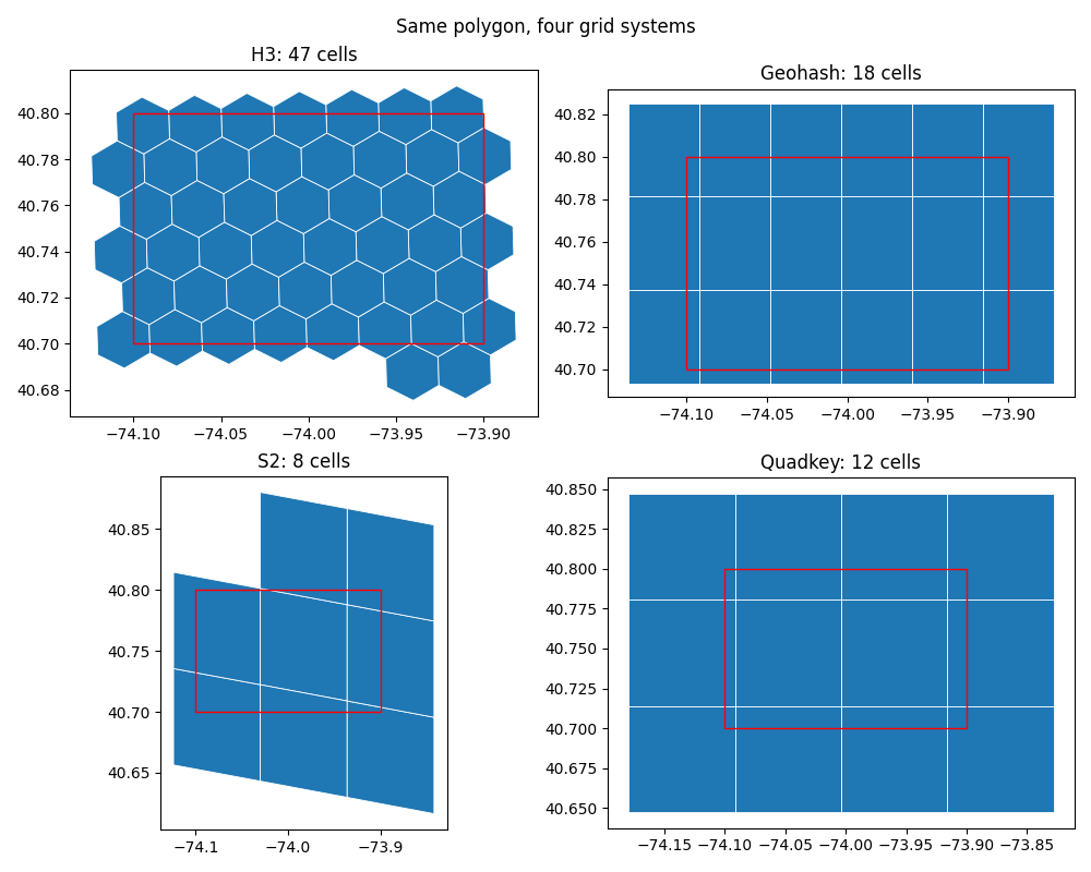
Example 6: Find optimal precision for your data

For best results with large areas, find precision explicitly first.

# Target ~100 cells
precision = m3s.S2.find_precision(polygon, method=100)
cells_100 = m3s.S2.from_geometry(polygon, precision=precision)
print(f"Using precision {precision}: {len(cells_100)} cells")

# Minimize coverage variance ('auto' method - recommended for quality)
precision_auto = m3s.H3.find_precision(polygon, method="auto")
print(f"Auto precision (minimize variance): {precision_auto}")

Using precision 12: 55 cells
Auto precision (minimize variance): 8

Example 7: The precision ladder, visualised

method='less' favours fewer, larger cells; 'auto' minimises coverage variance; 'more' favours finer cells.

fig, axes = plt.subplots(1, 3, figsize=(12, 4))
for ax, method in zip(axes, ("less", "auto", "more"), strict=True):
    p = m3s.H3.find_precision(polygon, method=method)
    method_cells = m3s.H3.from_geometry(polygon, precision=p)
    method_cells.plot(ax=ax, edgecolor="white", linewidth=0.6)
    outline.plot(ax=ax, color="red", linewidth=1)
    ax.set_title(f"method='{method}' → P{p}, {len(method_cells)} cells")
fig.suptitle("find_precision() methods on the same polygon")
plt.tight_layout()

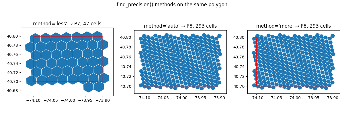
Example 8: Work with specific precision using with_precision()

cells_mgrs = m3s.MGRS.with_precision(5).from_geometry(
    (-74.1, 40.7, -73.9, 40.8)  # Bbox tuple (min_lon, min_lat, max_lon, max_lat)
)
result_gdf = cells_mgrs.to_gdf()
print(f"Created GeoDataFrame with {len(result_gdf)} MGRS cells")

Created GeoDataFrame with 358801 MGRS cells

Example 9: Get neighbors — rings around a cell

neighbors(cell, depth) returns the origin plus rings of surrounding cells. Hexagons make the rings obvious.

center = m3s.H3.from_geometry((-74.0060, 40.7128))
ring1 = m3s.H3.neighbors(center, depth=1)
ring2 = m3s.H3.neighbors(center, depth=2)
print(f"depth=1: {len(ring1)} cells, depth=2: {len(ring2)} cells")

ax = ring2.plot(facecolor="#c6dbef", edgecolor="white")
ring1.plot(ax=ax, facecolor="#6baed6", edgecolor="white")
m3s.H3.neighbors(center, depth=0).plot(ax=ax, facecolor="#2171b5", edgecolor="white")
ax.set_title("H3 neighbors: origin (dark) with depth-1 and depth-2 rings")
plt.tight_layout()

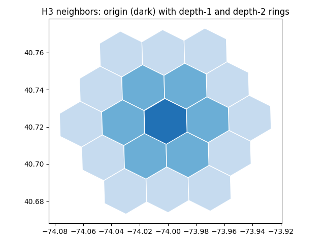
depth=1: 7 cells, depth=2: 19 cells

Example 10: Convert between grid systems — and see what conversion means

Default conversion uses the centroid method (fast, good for most cases). Below, the Geohash cells are filled and the converted H3 cells drawn on top.

geohash_cell = m3s.Geohash.from_geometry((-74.0, 40.7))
geohash_cells = m3s.Geohash.neighbors(geohash_cell)
h3_cells = geohash_cells.to_h3()  # Centroid method (default)
print(f"Converted {len(geohash_cells)} Geohash -> {len(h3_cells)} H3")

ax = geohash_cells.plot(facecolor="#fee391", edgecolor="white")
h3_cells.to_gdf().boundary.plot(ax=ax, color="#7a0177", linewidth=1.2)
ax.set_title("Geohash cells (filled) converted to H3 (purple outlines)")
plt.tight_layout()

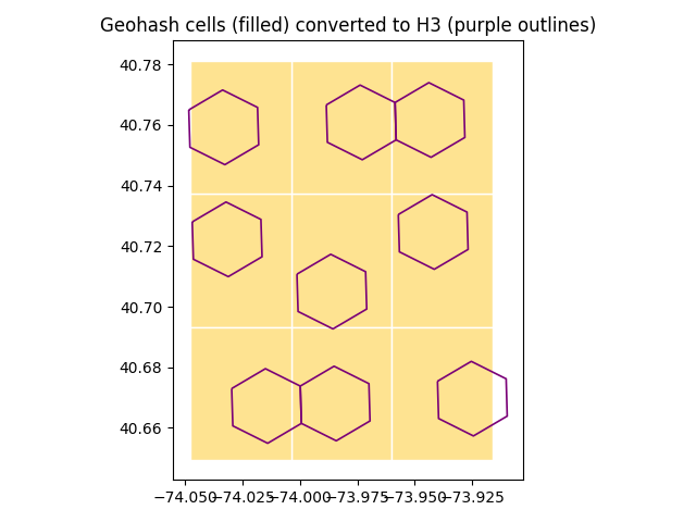
Converted 9 Geohash -> 9 H3

Example 11: Explicit conversion method if needed

h3_cells_overlap = geohash_cells.to_h3(method="overlap")  # More accurate
print(f"With overlap method: {len(h3_cells_overlap)} H3 cells")

With overlap method: 77 H3 cells

Example 12: Precision for use cases

precision = m3s.H3.find_precision_for_use_case("neighborhood")
cells_uc = m3s.H3.with_precision(precision).from_geometry(
    (-74.1, 40.7, -73.9, 40.8)  # Bbox (min_lon, min_lat, max_lon, max_lat)
)
print(f"Neighborhood-level precision {precision}: {len(cells_uc)} cells")

# Other use cases: 'building', 'block', 'city', 'region', 'country'
building_precision = m3s.Geohash.find_precision_for_use_case("building")
city_precision = m3s.S2.find_precision_for_use_case("city")
print(f"Building precision: {building_precision}")
print(f"City precision: {city_precision}")

Neighborhood-level precision 9: 1870 cells
Building precision: 8
City precision: 16

Example 13: Specific geometry methods when clarity is preferred

cell = m3s.MGRS.from_point(-74.0060, 40.7128)  # Explicit point method (lon, lat)
cells_bbox = m3s.S2.from_bbox((-74.1, 40.7, -73.9, 40.8))  # Explicit bbox method
cells_poly = m3s.Quadkey.from_polygon(polygon)  # Explicit polygon method

print(f"Used specific methods: {len(cells_poly)} Quadkey cells")

Used specific methods: 12 Quadkey cells

Example 14: Collection operations

GridCellCollection provides convenient operations

cells = m3s.H3.from_geometry(polygon, precision=7)

# Filter cells by area
large_cells = cells.filter(lambda c: c.area_km2 > 5.0)
print(f"Filtered to {len(large_cells)} cells > 5 km²")

# Convert to different formats
ids_list = cells.to_ids()
polygons_list = cells.to_polygons()
gdf = cells.to_gdf(include_utm=True)
print(f"Converted to {len(ids_list)} IDs, {len(polygons_list)} polygons")

Filtered to 47 cells > 5 km²
Converted to 47 IDs, 47 polygons

Example 15: Advanced workflow with chaining

# Complex workflow: geometry → cells → neighbors → convert → export
result = (
    m3s.H3.from_geometry(polygon, precision=7)
    .filter(lambda c: c.area_km2 > 3.0)
    .to_geohash()
)
print(f"Chained workflow result: {len(result)} cells")

Chained workflow result: 47 cells

Summary

M3S provides: 1. Direct access: m3s.H3, m3s.Geohash, m3s.S2, etc. (no instantiation needed) 2. Universal from_geometry(): handles any geometry type 3. Auto-precision: intelligent defaults based on coverage optimization 4. Easy conversions: .to_h3(), .to_geohash(), etc. 5. Visual checks: .plot() for figures, .explore() for interactive maps

print("\n" + "=" * 60)
print("M3S is easy to use without sacrificing power!")
print("=" * 60)

============================================================
M3S is easy to use without sacrificing power!
============================================================