Grid system enhancements

Three cross-system tools that build on the individual grids:

1. Conversion — map a cell from one grid system to another.

2. Relationship analysis — adjacency / containment between cells.

3. Multi-resolution — work across several precision levels at once.

The script runs top to bottom so every section renders its output (and plots) in the gallery.

import geopandas as gpd
import matplotlib.pyplot as plt
import numpy as np
from shapely.geometry import Point

from m3s import (
    GeohashGrid,
    H3Grid,
    QuadkeyGrid,
    analyze_relationship,
    convert_cell,
    create_adaptive_grid,
    create_adjacency_matrix,
    create_conversion_table,
    create_multiresolution_grid,
    find_adjacent_cells,
    list_grid_systems,
)

# Colorblind-safe palette (Okabe-Ito), shared across the figures below.
BLUE, ORANGE, GREEN = "#0072B2", "#E69F00", "#009E73"

1. Grid conversion

List the available systems, then convert a single Geohash cell into H3 and Quadkey using the centroid method.

systems_info = list_grid_systems()
print("Available grid systems:")
print(systems_info[["system", "default_precision", "default_area_km2"]].head())

source_cell = GeohashGrid(precision=5).get_cell_from_point(40.7128, -74.0060)
print(
    f"\nSource Geohash cell: {source_cell.identifier} ({source_cell.area_km2:.2f} km²)"
)

h3_cell = convert_cell(source_cell, "h3", method="centroid")
quadkey_cell = convert_cell(source_cell, "quadkey", method="centroid")
print(f"  → H3:      {h3_cell.identifier}")
print(f"  → Quadkey: {quadkey_cell.identifier}")

# Build a conversion table for a small area (Geohash p5 → H3 p7).
bounds = (-74.01, 40.71, -74.00, 40.72)  # (min_lon, min_lat, max_lon, max_lat)
conversion_table = create_conversion_table(
    "geohash", "h3", bounds, source_precision=5, target_precision=7
)
print(f"\nConversion table (Geohash → H3): {len(conversion_table)} mappings")
print(conversion_table.head())

Available grid systems:
    system  default_precision  default_area_km2
0       a5                  9        129.716396
1  geohash                  5         16.877753
2     mgrs                  1         99.857129
3       h3                  7          5.148941
4  quadkey                 12         47.762683

Source Geohash cell: dr5re (18.10 km²)
  → H3:      872a1072effffff
  → Quadkey: 032010110123

Conversion table (Geohash → H3): 2 mappings
  source_system source_id  ...  target_precision conversion_method
0       geohash     dr5re  ...                 7          centroid
1       geohash     dr5rs  ...                 7          centroid

[2 rows x 7 columns]

2. Relationship analysis

Take neighbouring Geohash cells and inspect adjacency between them.

cells = GeohashGrid(precision=6).get_cells_in_bbox(40.71, -74.01, 40.72, -74.00)
print(f"Analyzing relationships for {len(cells)} cells")

if len(cells) >= 2:
    relationship = analyze_relationship(cells[0], cells[1])
    print(f"First two cells are: {relationship.value}")

    adjacent = find_adjacent_cells(cells[0], cells[1:])
    print(f"Cells adjacent to the first: {len(adjacent)}")

    sample_cells = cells[: min(5, len(cells))]
    adj_matrix = create_adjacency_matrix(sample_cells)
    total = adj_matrix.values.sum()
    possible = len(sample_cells) * (len(sample_cells) - 1)
    print(f"Network connectivity: {total / possible:.3f}" if possible else "n/a")

Analyzing relationships for 4 cells
First two cells are: touches
Cells adjacent to the first: 3
Network connectivity: 1.000

3. Multi-resolution operations

A single grid driven at several precision levels, with hierarchy and adaptive subdivision.

base_grid = GeohashGrid(precision=5)
levels = [4, 5, 6, 7]
multi_grid = create_multiresolution_grid(base_grid, levels)

print("Resolution levels:")
print(multi_grid.get_resolution_statistics()[["level", "precision", "area_km2"]])

hierarchical = multi_grid.get_hierarchical_cells(Point(-74.0060, 40.7128))
print("\nHierarchical cells for NYC:")
for precision, cell in hierarchical.items():
    print(f"  precision {precision}: {cell.identifier} ({cell.area_km2:.2f} km²)")

region = (-74.02, 40.70, -73.98, 40.73)
multi_grid.populate_region(region)
transitions = multi_grid.analyze_scale_transitions(region)
print("\nScale transitions:")
print(transitions[["from_precision", "to_precision", "subdivision_ratio"]])

adaptive_gdf = create_adaptive_grid(base_grid, region, levels)
print(f"\nAdaptive grid: {len(adaptive_gdf)} cells")

Resolution levels:
   level  precision    area_km2
0      0          4  539.465713
1      1          5   16.877753
2      2          6    0.527607
3      3          7    0.016488

Hierarchical cells for NYC:
  precision 4: dr5r (579.34 km²)
  precision 5: dr5re (18.10 km²)
  precision 6: dr5reg (0.57 km²)
  precision 7: dr5regw (0.02 km²)

Scale transitions:
   from_precision  to_precision  subdivision_ratio
0               4             5                2.0
1               5             6               15.0
2               6             7               23.0

Adaptive grid: 90 cells

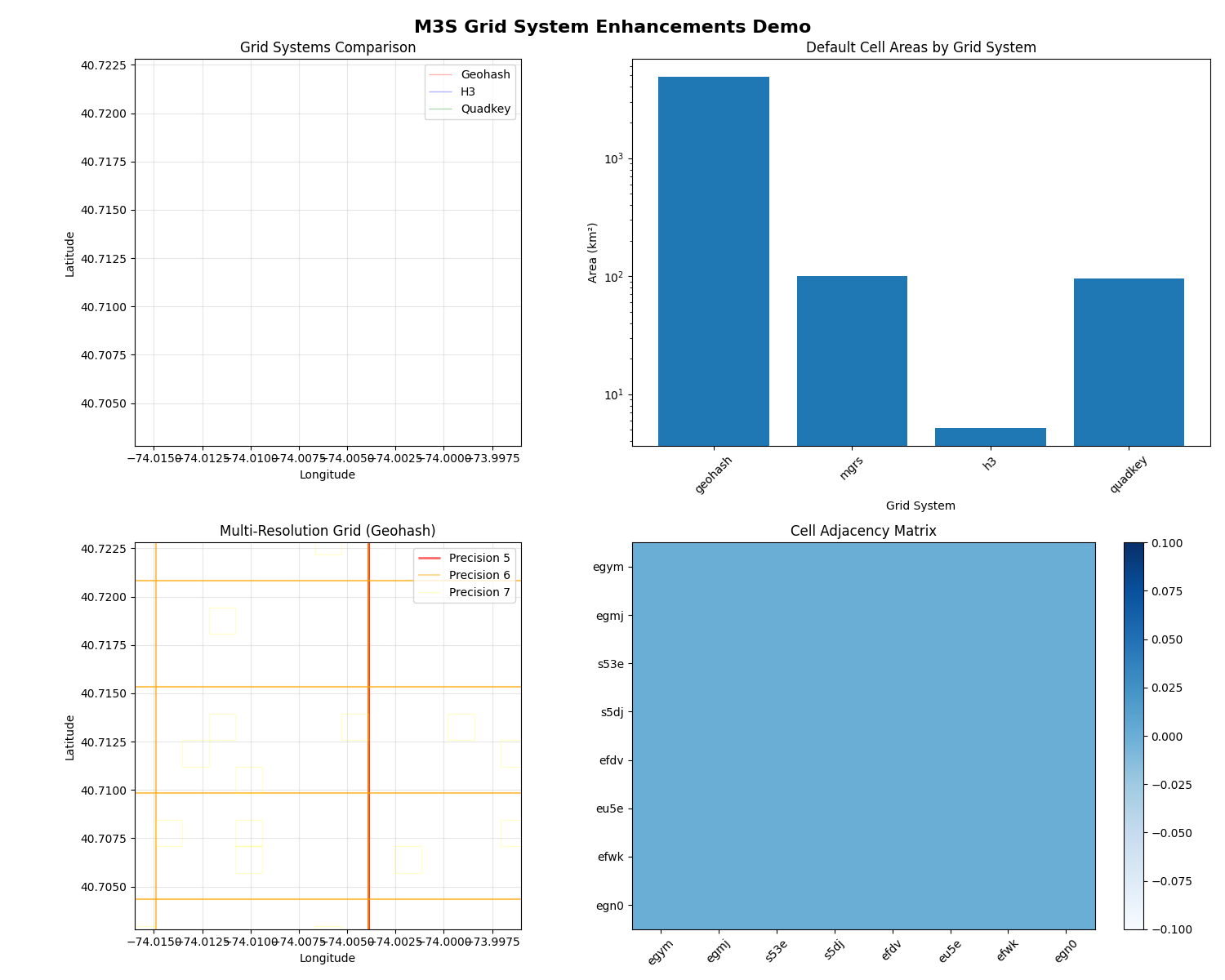
Visualising grid systems side by side

Geohash, H3 and Quadkey over the same small NYC window, plus their default cell areas and a multi-resolution overlay.

center_lon, center_lat = -74.0060, 40.7128
offset = 0.01
view = (
    center_lon - offset,
    center_lat - offset,
    center_lon + offset,
    center_lat + offset,
)

grids = {
    "Geohash": (GeohashGrid(precision=7), BLUE),
    "H3": (H3Grid(precision=9), ORANGE),
    "Quadkey": (QuadkeyGrid(precision=15), GREEN),
}

fig, axes = plt.subplots(2, 2, figsize=(13, 11))
fig.suptitle("M3S grid system enhancements", fontsize=15, fontweight="bold")

# (a) overlay of the three systems
ax = axes[0, 0]
ax.set_title("Grid systems overlay")
for name, (grid, color) in grids.items():
    cells_bbox = grid.get_cells_in_bbox(*view)[:20]
    if cells_bbox:
        gdf = gpd.GeoDataFrame({"geometry": [c.polygon for c in cells_bbox]})
        gdf.boundary.plot(ax=ax, color=color, linewidth=1.2, label=name)
ax.legend()
ax.set_xlim(view[0], view[2])
ax.set_ylim(view[1], view[3])
ax.set_axis_off()

# (b) default cell area by system
ax = axes[0, 1]
ax.set_title("Default cell area by system")
plot_systems = systems_info[
    systems_info["system"].isin(["geohash", "h3", "quadkey", "mgrs"])
]
ax.bar(plot_systems["system"], plot_systems["default_area_km2"], color=BLUE)
ax.set_ylabel("Area (km²)")
ax.set_yscale("log")
plt.setp(ax.get_xticklabels(), rotation=45)

# (c) multi-resolution overlay
ax = axes[1, 0]
ax.set_title("Multi-resolution (Geohash)")
level_cells = create_multiresolution_grid(base_grid, [5, 6, 7]).populate_region(view)
shades = [BLUE, ORANGE, GREEN]
for i, (precision, cells_lvl) in enumerate(level_cells.items()):
    if cells_lvl:
        gdf = gpd.GeoDataFrame({"geometry": [c.polygon for c in cells_lvl[:15]]})
        gdf.boundary.plot(
            ax=ax,
            color=shades[i],
            linewidth=2 - i * 0.5,
            label=f"precision {precision}",
        )
ax.legend()
ax.set_xlim(view[0], view[2])
ax.set_ylim(view[1], view[3])
ax.set_axis_off()

# (d) adjacency matrix heatmap
ax = axes[1, 1]
ax.set_title("Cell adjacency matrix")
sample = GeohashGrid(precision=8).get_cells_in_bbox(
    center_lat - 0.005, center_lon - 0.005, center_lat + 0.005, center_lon + 0.005
)[:8]
if len(sample) > 1:
    matrix = create_adjacency_matrix(sample)
    im = ax.imshow(matrix.values, cmap="Blues")
    labels = [c.identifier[-4:] for c in sample]
    ax.set_xticks(range(len(sample)), labels, rotation=45)
    ax.set_yticks(range(len(sample)), labels)
    fig.colorbar(im, ax=ax, fraction=0.046)
else:
    ax.text(0.5, 0.5, "Insufficient cells", ha="center", va="center")
    ax.set_axis_off()

plt.tight_layout()
plt.show()

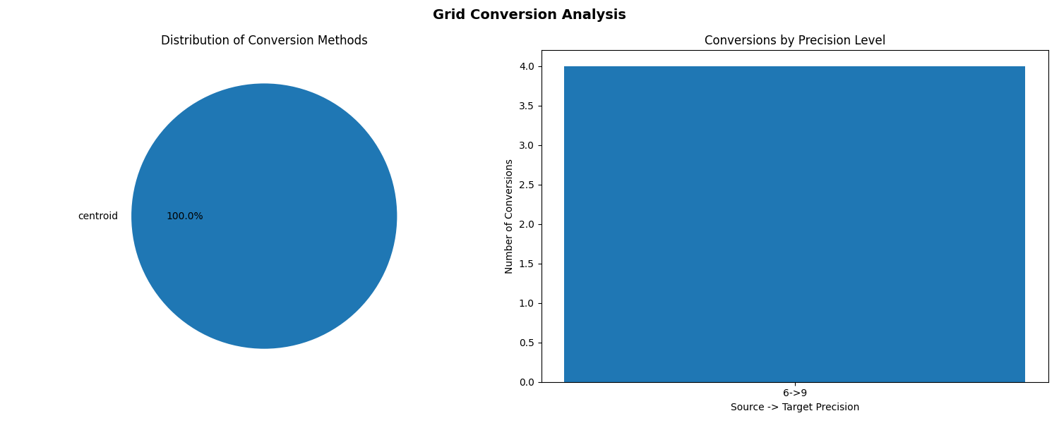
Conversion analysis

How a Geohash → H3 conversion over a region distributes across methods and precision pairs.

table = create_conversion_table(
    "geohash", "h3", bounds, source_precision=6, target_precision=9
)

if len(table) > 0:
    fig, (ax1, ax2) = plt.subplots(1, 2, figsize=(13, 5))
    fig.suptitle("Grid conversion analysis", fontsize=14, fontweight="bold")

    method_counts = table["conversion_method"].value_counts()
    ax1.pie(
        method_counts.values,
        labels=method_counts.index,
        autopct="%1.1f%%",
        colors=[BLUE, ORANGE, GREEN],
    )
    ax1.set_title("Conversion methods")

    pairs = (
        table.groupby(["source_precision", "target_precision"])
        .size()
        .reset_index(name="n")
    )
    ax2.bar(np.arange(len(pairs)), pairs["n"], color=BLUE)
    ax2.set_xticks(
        np.arange(len(pairs)),
        [f"{r.source_precision}→{r.target_precision}" for r in pairs.itertuples()],
    )
    ax2.set_title("Conversions by precision pair")
    ax2.set_ylabel("Count")

    plt.tight_layout()
    plt.show()